April 24, 2024

Statistics in SQL Server

This post is a quick introduction to statistics in SQL Server.

SQL Server maintains statistics about the volume and distribution of data in columns and indexes. The optimizer uses these statistics when it creates a query execution plan. They help it with the task of cardinality estimation, i.e. estimating how many rows will be processed by operators in a plan. These estimates influence the decisions made by the optimizer, like which data access mechanism to use, e.g. scan or seek. These decisions can be the difference between an optimal plan and a sub-optimal plan.

For the most part SQL Server handles the maintenance of statistics for you. It creates them by default: automatically on columns that are used in a filtering capacity (JOIN, WHERE, or HAVING clauses) and automatically on indexes when they are created. They are also updated automatically after a certain number of modifications have occurred. It's a best practice to leave these settings alone.

What are the statistics?

Statistics are stored as objects in SQL Server and they have three parts: a header, a density vector and a histogram. The header contains high level metadata, e.g. when the statistics were created, how many rows were sampled. The density vector is information about the average number of duplicates in the column(s). Density is calculated as 1 / the number of distinct values in a column(s). 100% is the most dense meaning all values are the same. The histogram is a bucketized representation of the index or column, and if it's a multi-column index or statistic then it's always the leading column.

Viewing statistics objects

You can see the statistics using DBCC SHOW_STAISTICS(table_or_index, stats_name). Here it is used to show the statistics on the AK_Product_Name index of the Production.Product table in AdventureWorks:

DBCC SHOW_STATISTICS
(
    'Production.Product', 
    AK_Product_Name
)

DBCC SHOW_STATISTICS

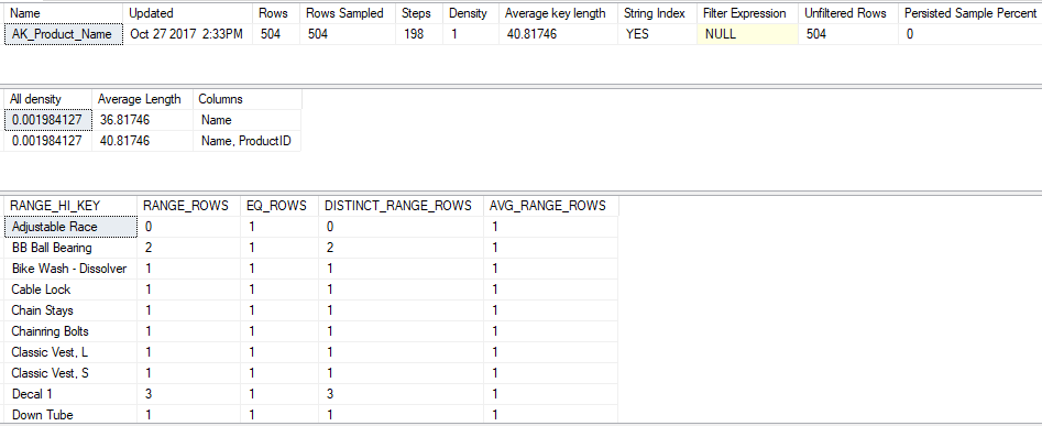
The top result is the header, followed by the density vector and the histogram. The header is pretty self-explanatory. Rows Sampled is the sample size used to create the statistics. A sample is obviously faster than doing a FULLSCAN of the table but since there are only 504 rows in this index it did a FULLSCAN. The Density in the header can be ignored because it's for backwards compatibility.

Density vector

There are two rows in the density vector for the AK_Product_Name index. The first row shows the density on the Name column, which is the only column in the index. The second row shows the combined density of Name and ProductID (ProductID is the clustering key). The clustering key is included in the density vector on clustered tables because it's part of the non-clustered index.

Both the Name column on its own and the combination of Name and ProductID columns have the same density value of 0.001984127. It's because this is a unique index on Name therefore Name cannot have a higher density than the combined Name and ProductID.

The density value is easily checked by doing 1 divided by the number of distinct (Name) or (Name, ProductID) values in the table:

--Density for (Name)
SELECT 1.0 / 
COUNT(DISTINCT [Name]) AS NameDensity 
FROM Production.Product

--result
--0.001984126984

--Density for (Name, ProductID)
SELECT 1.0 / COUNT(*) 
FROM
(
    SELECT DISTINCT 
    [Name], ProductID AS NameDensity 
    FROM Production.Product
) AS a

--result
--0.001984126984

Density and Selectivity

Density is closely related to selectivity. Selectivity is what a predicate has: it's the expected ratio of matching rows for the predicate. It helps me to picture this as an inverse relationship:

stats-density

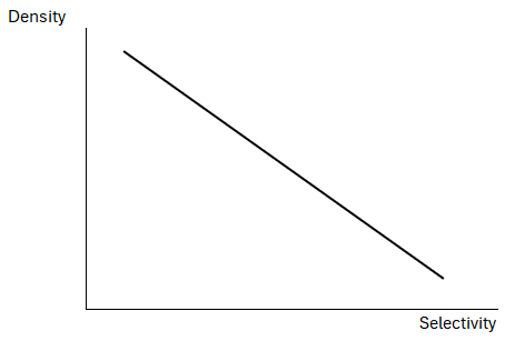
Imagine a Car table with millions of rows and two of its columns are LicencePlate and Make. Licence plates are unique so the column LicencePlate has a low density (1 / number of distinct values); it's actually a good primary key candidate. This means a predicate on LicencePlate will be highly selective so it should just return one row! Make on the other hand has a higher density because it has a lot of duplicates (lots of cars have the same make). This means predicates on Make won't be as selective as a predicates on LicensePlate, i.e. the expected ratio of matching rows will be a lot more than 1, e.g., you'd expect the predicate WHERE Make = 'Ford' to match a lot of rows.

The optimizer uses the density vector to estimate cardinality under certain conditions, e.g. when using a local variable in a predicate. For example the Production.TransactionHistory table in AdventureWorks2019 has an index (IX_TransactionHistory_ProductID) on ProductID. When a local variable is used in the WHERE clause the optimizer uses the density vector to estimate the cardinality:

DECLARE @ProductID INT = 784

SELECT * 
FROM [Production].[TransactionHistory] 
WHERE ProductID = @ProductID
GO

stats-density

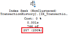
The estimated number of rows is 257. Running DBCC SHOW_STATISTICS:

DBCC SHOW_STATISTICS
(
    'Production.TransactionHistory', 
    IX_TransactionHistory_ProductID
)

stats-density

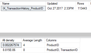
The 257 estimate is the result of multiplying the density (0.002267574) by the cardinality (113,443) of the index:

SELECT 0.002267574 * 113443

--result
--257.240397282

Histogram

A histogram shows the distribution of data in a column. It normally looks like a bar chart but SQL Server histograms are tabular. The histogram part of a statistics object is always created on one column, the leading column of an index or multi-column statistic. It puts the data in buckets (up to 200) and counts the frequency of the values on and in between the steps.

stats-density

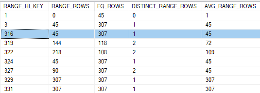
The above histogram shows the distribution of values in the ProductID column of the IX_TransactionHistory_ProductID index on the Production.TransactionHistory table. The first column (RANGE_HI_KEY) contains actual values from the column. The other columns contain information about the number rows at and between the bucket boundaries. For example, consider the step where RANGE_HI_KEY is 316. From the histogram SQL Server knows that:

EQ_ROWS: 307 values match the predicate ProductID = 316
RANGE_ROWS: 45 values are within the range defined by the previous bucket item (3) and the current item (316), exclusively, ProductID > 3 AND ProductID < 316
- DISTINCT_RANGE_ROWS: There is 1 distinct value in the same exclusive range
- AVG_RANGE_ROWS: the average number of values equal to any potential key value within the range is 45

The histogram is the the most important statistic. It's the first place the optimizer gets its estimates from.

Conclusion

So that's a very basic overview of statistics in SQL Server. They're used by the optimizer to help make its cost-based decision on which execution plan to use. Topics like how statistics can negatively impact performance will be covered in a future post.