Learning PySpark Part 2: The DataFrame API
This is part 2 of a series about learning PySpark (Spark 3.5.3) the Python API for Apache Spark (referred to as Spark from now on). In part 1 I showed you how to get started by using Docker to setup a Spark cluster locally. Containers are ideal for learning Spark and PySpark because they are isolated environments that can be created and deleted as required.
This part will be a high-level introduction to the DataFrame API, which is one of the APIs for working with structured data (the other is DataSets, which isn't supported in PySpark). The coverage won't be exhaustive as it would be too long (and boring). The aim of parts 2 and 3 is to introduce just enough of the API to gain a working knowledge of PySpark. At the end of part 3 you will be able to translate between SQL and PySpark. After some practice it'll be second nature. This is my ongoing goal. Coming from a SQL background I wanted to get to a point where transforming data in Python (with PySpark) is as familiar to me as doing it in SQL.
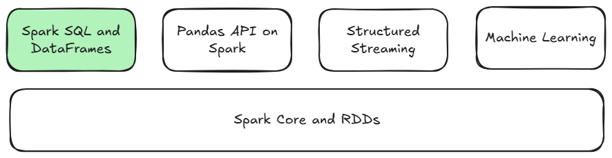
Spark the unified platform
Spark is a unified platform, which means it supports a range of use cases, like batch processing, stream processing, and machine learning, among others. With PySpark it's possible to create Spark applications that use one or all of the main Spark features. The scope of this series, however, is limited to the DataFrame API.
You should learn how Spark works
If you're completely new to Spark you should at least learn the basics about how it works. Just learning a high-level API like PySpark won't give you a conceptual idea of how all the moving parts interact when a Spark application runs.
I attempted to write a small section about how Spark works but it was impossible to keep it short enough without it being oversimplified and, therefore, pointless. Apologies. Search and you'll find plenty of good explanations online. And for detailed coverage I recommend a book, like Spark: The Definitive Guide.
Overview of a PySpark program
At a high level, a PySpark program will have these parts:
- An instance of
SparkSessionto be used as the entry point to the DataFrame API. - The loading of data from sources into DataFrames.
- Transformations applied to DataFrames to create new DataFrames.
- Writing the transformed results to a destination.
The structure of this post will roughly follow the above sequence. Before we can do anything in PySpark we need an entry point, which is covered in the next section. After that I'll introduce DataFrames and create a toy example with dummy data. Then I'll explain how to load data sources, followed by a brief look at transforming data (which is the topic of part 3), and finally I'll end on writing data to a destination.
Create an entry point
To follow along have a Spark cluster ready in a Docker container and a Jupyter notebook ready to receive and run the examples. See part 1 for details.
The first thing to do when writing a PySpark program is to create an instance of the SparkSession class. It will serve as the entry point through which functionality of the DataFrame API can be accessed. Import SparkSession and create an instance of it called spark:
from pyspark.sql import SparkSession

spark = SparkSession \
    .builder \
    .appName("My first PySpark App") \
    .getOrCreate()
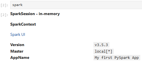
The builder pattern is used to create the spark variable. We've given the Spark application a name with appName() and created it with getOrCreate(). There are other settings but we won't cover those yet.
You probably won't have to create a SparkSession in your day to day job as a data engineer because in the managed services that you'll be using, like Azure Databricks, the SparkSession is created for you.
Calling the spark variable displays information about the Spark application:
Introducing DataFrames
A DataFrame is a data structure for storing and transforming data that is organised into rows and columns, i.e., structured data. The DataFrame API provides lots of ways to transform structured data: selecting, filtering, joining, aggregating, and windowing. This will sound familiar if you have a SQL background, and that's because the Spark SQL module and the DataFrame API are both interfaces for working with structured data.
Spark SQL, as the name suggests, is used to transform data using SQL whereas the DataFrame API is used to transform data using a programming language, in our case Python. But under the hood it's the same execution engine, so it's possible to switch between (and mix) the two APIs depending on which is more suitable. A transformation defined with DataFrames can be converted to SQL, and vice versa.
Creating a DataFrame
Let's create a very simple DataFrame. Run the following in your notebook:
data = [
    (1, 'Bob', 44, 'Economics'),
    (2, 'Alice', 47, 'Science'),
    (3, 'Tim', 28, 'Science'),
    (4, 'Jane', 33, 'Economics')
]

columns = ['id', 'name', 'age', 'subject']

students = spark.createDataFrame(data, columns)
We define some dummy data using native Python types. The data variable is a list of tuples. Each tuple will become a row in the DataFrame and each value in the tuple will become a column in that row. The column names are a list of strings in the columns variable. We've used the spark variable (the entry point to Spark functionality, remember) to expose the DataFrame API. It gave us access to the createDataFrame() method, to which we passed the data and columns variables. The resulting DataFrame is stored in the students variable.
Confirm the students variable is a DataFrame:
type(students)
Output:
pyspark.sql.dataframe.DataFrame
The contents of a DataFrame can be displayed by using its show() method:
students.show()
Output:
+---+-----+---+---------+
| id| name|age|  subject|
+---+-----+---+---------+
|  1|  Bob| 44|Economics|
|  2|Alice| 47|  Science|
|  3|  Tim| 28|  Science|
|  4| Jane| 33|Economics|
+---+-----+---+---------+
Some useful DataFrame properties and methods
The full list is found in the API reference but here's a quick look at some DataFrame properties and methods I use often.
List columns
A DataFrame has a columns property that returns a list of columns:
students.columns
Output:
['id', 'name', 'age', 'subject']
In part 3 we'll retrieve the columns like this in order to do a dynamic pivot—a transformation that I think is better expressed in DataFrame code rather than SQL.
Count rows
Count the number of rows with the count() method:
students.count()
Output:
4
Create a temporary view
This series is focused on the DataFrame API but you'll sometimes find that SQL is more appropriate to express a transformation. Furthermore it's not unusual to find SQL mixed in with DataFrame code. You can switch to SQL by using the sql property of the SparkSession variable.
The following creates a temporary view with the students DataFrame:
students.createOrReplaceTempView("vw_students")
This allows us to use SQL on the DataFrame:
spark.sql("SELECT * FROM vw_students WHERE name = 'Bob';").show()
Output:
+---+----+---+---------+
| id|name|age|  subject|
+---+----+---+---------+
|  1| Bob| 44|Economics|
+---+----+---+---------+
Schemas
DataFrames are like SQL tables. They have rows and columns, and each column has the same number of rows. They also have a schema that defines the data types of its columns. The DataFrame's printSchema() method does just that:
students.printSchema()
Output:
root
 |-- id: long (nullable = true)
 |-- name: string (nullable = true)
 |-- age: long (nullable = true)
 |-- subject: string (nullable = true)
Another option is to use a DataFrame's schema attribute to return the schema as a StructType:
students.schema
Output:
StructType([StructField('id', LongType(), True), StructField('name', StringType(), True), StructField('age', LongType(), True), StructField('subject', StringType(), True)])
A schema is a StructType that contains a StructField type for each column. The StructType is iterable, allowing it to be looped over, like this:
for column in students.schema:
    print(column)

for column in students.schema:
    print(column.dataType)
Output:
StructField('id', LongType(), True)
StructField('name', StringType(), True)
StructField('age', LongType(), True)
StructField('subject', StringType(), True)

StringType()
LongType()
StringType()
This tells us that the id column is of the LongType and is nullable, as indicated by the Boolean.
Defining a schema manually
A schema can be defined before the DataFrame is created. This approach is recommended if you know the types of the data source because reading the entire data source to infer types can be an expensive operation:
from pyspark.sql.types import StructType, StructField
from pyspark.sql.types import IntegerType, StringType

schema = StructType([
    StructField('id', IntegerType(), True),
    StructField('name', StringType(), True),
    StructField('age', IntegerType(), True),
    StructField('subject', StringType(), True)
])

students = spark.createDataFrame(data, schema)

students.printSchema()
Output:
root
 |-- id: integer (nullable = true)
 |-- name: string (nullable = true)
 |-- age: integer (nullable = true)
 |-- subject: string (nullable = true)
Notice how when students was created without explicitly using a schema (i.e., when we just used a list of column names), Spark chose the LongType for the id and age columns. But here we've declared explicitly that they should be the IntegerType.
You might also be wondering why the second parameter to createDataFrame() went from being a list of strings in the column variable to the schema variable, which is a StructType. This is perfectly fine. If you look in the documentation, it confirms that the schema parameter accepts several patterns, including a list of column names or a StructType (i.e., an explicit schema). You will find a lot of flexibility like this in the PySpark API.
Define a schema with DDL
The example above was quite verbose. A clearer way of defining a schema is to use data definition language (DDL):
schema = "id INT, name STRING, age INT, subject STRING"
students = spark.createDataFrame(data, schema)
Data types
Spark has its own type system. I won't list the types as they can be looked up (here and here) easily enough, but it's worth remembering a few things. Types are imported from the pyspark.sql.types module. There are simple types, like IntegerType(), FloatType(), StringType(), BooleanType(), which correspond to the Python types int, float, str, bool, respectively.
And then there are complex types, like DateType() (datetime.date), TimestampType() (datetime.datetime), StructType (dict), and ArrayType(elementType) (list) (the Python type is in brackets).
Partitions
Spark, being the distributed engine that is it, splits DataFrames into partitions that are shared amongst the nodes in a cluster. You have to remember that in a real world application, a DataFrame may be too big to fit in the memory of a single machine, so to process it efficiently it must be broken up into chunks and distributed across a cluster of machines. That's the whole point of Spark.
Luckily the PySpark programmer doesn't need to worry about managing partitions and can instead focus on transforming data using high-level abstractions, like DataFrames.
In memory and lazy evaluation
A few more things to mention about DataFrames and, really, Spark in general. Spark is fast because it computes everything in-memory (unlike its predecessor, Hadoop MapReduce). There's a lot more to it but that's the key thing: "in-memory".
Finally, Spark uses lazy evaluation meaning it doesn't compute the results of a transformation until triggered to do so by an action. This code aggregates sales by month (don't run it because we haven't actually created a sales_df):
monthly_sales = (
    sales_df
    .groupBy('Month')
    .agg(
        sum('Sales').alias('Sales')
    )
)
But the monthly_sales DataFrame doesn't contain any data. Rather, it stores a representation of the transformation steps (grouping and aggregating, as well those that created sales_df) required to compute the monthly_sales DataFrame. The fancy term for this representation is a directed acyclic graph (DAG). The transformations are physically executed on underlying data only after an action, such as show(), is called. So only at the very last minute will it compute a result and show some data.
Lazy evaluation allows Spark to optimize the plan, with techniques like predicate pushdown.
That covers the basics of DataFrames. Next, we will see how to load a data source.
Loading data
This section is about loading data from a data source. There are lots of different data sources. There are a handful of built in ones, like CSV, Parquet, and JSON, and then there are many more third party ones authored by the community, like MongoDB.
How is data loaded into a DataFrame? Everything begins at the entry point, the spark variable, which is an instance of SparkSession. It has a read property that returns a DataFrameReader, and it's through this type that we can read data into DataFrames.
In PySpark you'll find that there are multiple ways of doing the same thing, including reading from data sources. One pattern uses the DataFrameReader method that has the same name as the data source, e.g., csv, parquet, json, jdbc, orc, text. These are the built in ones:
# csv
spark.read.csv("./path/to/some-data.csv", <options>)

# parquet
spark.read.parquet("./path/to/some-data.csv", <options>)

# and others, like json, jdbc, orc, text
These methods return a DataFrame. Parameters set various options, e.g., commonly used options for reading a CSV file are header and inferSchema.
The other pattern for reading data sources uses the format() method of the DataFrameReader class. It takes the data source as a string, e.g., "csv" and returns another DataFrameReader. Options are set as key/value pairs using the DataFrameReader.option("key", "value") method. option() returns a DataFrameReader meaning multiple options can be set by chaining together calls to the option() method. And finally, the load() method returns a DataFrame.
df = spark.read\
    .format("...")\ # e.g., "csv", "parquet", "json"
    .option("key", "value")\
    .option("key", "value")\
    .load("./path/to/some-data.csv")
CSV example
Here's an example of reading a CSV file into a DataFrame. Download the Titanic dataset if you don't have a CSV file to practice with. Place it in the folder that was set as the host path of the volume when the container was created (-v "host-path:container-path"). Let's say you set the volume (-v) as follows:
docker run
...
-v "C:\work\spark:/home/jovyan/work"
...
So you would put the CSV file in the C:\work\spark folder.
Now we can read the file into a DataFrame. Here's one way of doing it:
titanic_df = spark.read.csv("titanic.csv")

titanic_df.show(2)
Notice I limited the number of displayed records by passing an integer to the show() method:
+-----------+--------+------+--------------------+----+---+-----+-----+---------+----+-----+--------+
|        _c0|     _c1|   _c2|                 _c3| _c4|_c5|  _c6|  _c7|      _c8| _c9| _c10|    _c11|
+-----------+--------+------+--------------------+----+---+-----+-----+---------+----+-----+--------+
|PassengerId|Survived|Pclass|                Name| Sex|Age|SibSp|Parch|   Ticket|Fare|Cabin|Embarked|
|          1|       0|     3|Braund, Mr. Owen ...|male| 22|    1|    0|A/5 21171|7.25| NULL|       S|
+-----------+--------+------+--------------------+----+---+-----+-----+---------+----+-----+--------+
We can see that the header has been read as a row of data. To correct this set the header option to True:
titanic_df = spark.read.csv("titanic.csv", header=True)
titanic_df.show(2)
Output:
+-----------+--------+------+--------------------+------+---+-----+-----+---------+-------+-----+--------+
|PassengerId|Survived|Pclass|                Name|   Sex|Age|SibSp|Parch|   Ticket|   Fare|Cabin|Embarked|
+-----------+--------+------+--------------------+------+---+-----+-----+---------+-------+-----+--------+
|          1|       0|     3|Braund, Mr. Owen ...|  male| 22|    1|    0|A/5 21171|   7.25| NULL|       S|
|          2|       1|     1|Cumings, Mrs. Joh...|female| 38|    1|    0| PC 17599|71.2833|  C85|       C|
+-----------+--------+------+--------------------+------+---+-----+-----+---------+-------+-----+--------+
The header is now where it should be. Let's look at the schema:
titanic_df.printSchema()
Output:
root
 |-- PassengerId: string (nullable = true)
 |-- Survived: string (nullable = true)
 |-- Pclass: string (nullable = true)
 |-- Name: string (nullable = true)
 |-- Sex: string (nullable = true)
 |-- Age: string (nullable = true)
 |-- SibSp: string (nullable = true)
 |-- Parch: string (nullable = true)
 |-- Ticket: string (nullable = true)
 |-- Fare: string (nullable = true)
 |-- Cabin: string (nullable = true)
 |-- Embarked: string (nullable = true)
The CSV reader assigned every column the StringType, but we can see that there are some integers and doubles. Set the inferSchema option to True so that Spark reads the entire CSV file to determine the types. Keep in mind this operation can be slow for big files:
titanic_df = spark.read.csv("titanic.csv", header=True, inferSchema=True)
titanic_df.printSchema()
Output:
root
 |-- PassengerId: integer (nullable = true)
 |-- Survived: integer (nullable = true)
 |-- Pclass: integer (nullable = true)
 |-- Name: string (nullable = true)
 |-- Sex: string (nullable = true)
 |-- Age: double (nullable = true)
 |-- SibSp: integer (nullable = true)
 |-- Parch: integer (nullable = true)
 |-- Ticket: string (nullable = true)
 |-- Fare: double (nullable = true)
 |-- Cabin: string (nullable = true)
 |-- Embarked: string (nullable = true)
Now the columns have suitable types.
Parquet example
The New York Taxi & Limousine Commission (TLC) publishes trip record data for anyone to download and use. These datasets are in the Parquet format. Download one and move it to the same folder as the CSV file (host volume path) so it can be read into a DataFrame.
This time I will use the format() method of the read property:
tlc_df = (spark
    .read
    .format("parquet")
    .load("yellow_tripdata_2025-01.parquet")
)
Let's look at some properties of this DataFrame.
print(tlc_df.count())

tlc_df.columns
Output:
3475226

['VendorID',
 'tpep_pickup_datetime',
 'tpep_dropoff_datetime',
 'passenger_count',
 'trip_distance',
 'RatecodeID',
 'store_and_fwd_flag',
 'PULocationID',
 'DOLocationID',
 'payment_type',
 'fare_amount',
 'extra',
 'mta_tax',
 'tip_amount',
 'tolls_amount',
 'improvement_surcharge',
 'total_amount',
 'congestion_surcharge',
 'Airport_fee']
Applying transformations
Now that we have a DataFrame we would then proceed to transform it. Transforming data is the topic of part 3 but here's a little taster.
DataFrame transformations are just a different way of expressing SQL transformations. Take this SQL query that returns the students aged 40 and over:
SELECT name
FROM student
WHERE age >= 40
The PySpark DataFrame equivalent of this SQL query is:
students.select('name').where('age >= 40').show()
Output:
+-----+
| name|
+-----+
|  Bob|
|Alice|
+-----+
show(), by the way, doesn't return a Dataframe, it returns None, so if you wanted to store this transformation in a variable and then perform more transformations later you would need to remove the show() method:
t1 = students.where('age >= 40').select('name') # show() removed

t2 = # some more transformations

t2.show()
Only use show() when you need to see the DataFrame because using it in the middle of a series of transformations will lead to incorrect results.
Writing data
Writing data has a similar pattern to reading data. To read (or load) data we used a DataFrameReader type obtained through the read property of the SparkSession variable spark. To write data we use the DataFrameWriter type obtained through the write property of a DataFrame. It makes sense that the interface (write) is gotten through the DataFrame rather than the SparkSession because the DataFrame is being written.
DataFrameWriter has methods for specifying how to write to storage. As with reading, there are several built in ones, like csv, parqet, json, orc, jdbc, and text. And there are many more third party ones. Alternatively the format can be specified as a string, .e.g., write.format("parquet").
Save modes
The save operation, the mode parameter, can be either:
appendoverwriteignore- silently ignore if existserror(default) throws an error if the data exists
Setting options
Options are set as key/value pairs using the DataFrameWriter 's option(key, value) method. Options set things like the separator when writing to CSV.
CSV Example
Here is an example of writing the student DataFrame to CSV.
students.write.csv("students", header=True, mode="overwrite")
Notice the path I used, "students", does not have the .csv extension. This is because Spark writes to a folder, not a single file, so the extension would look odd. If you look in the students folder you'll see several CSV files:
PS C:\Work\spark\students> dir *.csv -Name

part-00000-aa6d014b-8032-42ef-a3d6-01faceb60bd9-c000.csv
part-00002-aa6d014b-8032-42ef-a3d6-01faceb60bd9-c000.csv
part-00005-aa6d014b-8032-42ef-a3d6-01faceb60bd9-c000.csv
part-00008-aa6d014b-8032-42ef-a3d6-01faceb60bd9-c000.csv
part-00011-aa6d014b-8032-42ef-a3d6-01faceb60bd9-c000.csv
Each file represents a partition of the DataFrame.
If you wanted to merge the partitions and write to a single CSV file you could turn the Spark DataFrame into a Pandas DataFrame and then write it to a CSV file:
students.toPandas().to_csv("students.csv")
This is not recommended for large amount of data because merging the partitions is an expensive operation. I tried this on a 1M row DataFrame with a handful of columns and it ran out of memory. Granted, this was on my workstation, but still.
Conclusion of Part 2
In Part 2 I introduced the DataFrame API for working with structured data. A DataFrame is like a SQL table in that it has rows and columns and a schema that defines the column data types. DataFrames are not unique to Spark, for example, Pandas has them too. What makes the Spark DataFrame different is that it's designed to be partitioned across nodes in a cluster so that transformations can happen in parallel. This is how Spark can process massive amounts of data (imagine DataFrames that are terabytes in size) in a reasonable amount of time.
In Part 3 we will take a more detailed look at transforming data with the DataFrame API.